Problem set 2: Finite difference methods
Topics covered: Finite difference methods, boundary condition enforcement, stability.
Note: If you miss the problem solving class, you have to submit solutions to 1a)-d) and 2a)-b) in Studium before the deadline.
Preliminaries
Consider a uniform grid of \(m+1\) points, with grid spacing \(h = \frac{L}{m}\). Let \(\mathbf{e}_{\ell}\) and \(\mathbf{e}_r\) denote the following vectors in \(\mathbb{R}^{m+1}\):
\[\begin{split}
\mathbf{e}_{\ell} = \begin{bmatrix}
1 \\ 0 \\ \vdots \\ 0
\end{bmatrix},
\quad
\mathbf{e}_{r} = \begin{bmatrix}
0 \\ 0 \\ \vdots \\ 1
\end{bmatrix}.
\end{split}\]
Definition of \(D_1\)
A difference operator \(D_1\) is a first-derivative SBP operator with quadrature matrix \(H\) if \(H=H^T>0\) and
\[
HD_1 = \mathbf{e}_r \mathbf{e}_r^T - \mathbf{e}_\ell \mathbf{e}_\ell^T - D_1^T H .
\]
Definition of \(D_2\)
A difference operator \(D_2\) approximating
\(\partial^2/\partial\,x^2\) is a second-derivative SBP operator if
\[
HD_2 = \mathbf{e}_r \mathbf{d}_r^T - \mathbf{e}_{\ell} \mathbf{d}_\ell^T - M,
\]
where \(H=H^T>0\), \(M=M^T \ge 0\), and \(\mathbf{d}_\ell^T v\simeq u_x|_{x=0}\), \(\mathbf{d}_r^T v \simeq u_x |_{x=L}\) are finite difference approximations of the first derivatives at the left and right boundary points.
Discrete inner product
Let \((\cdot, \cdot)_H\) denote the discrete inner product, defined by
\[
(\mathbf{u}, \mathbf{v})_H = \mathbf{u}^* H \mathbf{v}.
\]
Note that \((\cdot, \cdot)_H\) approximates the \(L^2\) inner product \((\cdot, \cdot)\), since \(H\) is a quadrature operator. In the discrete inner product, the SBP operators satisfy
\[
(\mathbf{u}, D_1 \mathbf{v})_H = (\mathbf{e}_r^T \mathbf{u})^* (\mathbf{e}_r^T \mathbf{v}) - (\mathbf{e}_\ell^T \mathbf{u})^* (\mathbf{e}_\ell^T \mathbf{v}) - (D_1 \mathbf{u}, \mathbf{v})_H
\]
and
\[
(\mathbf{u}, D_2 \mathbf{v})_H = (\mathbf{e}_r^T \mathbf{u})^* (\mathbf{d}_r^T \mathbf{v}) - (\mathbf{e}_\ell^T \mathbf{u})^* (\mathbf{d}_\ell^T \mathbf{v}) - \mathbf{u}^* M \mathbf{v}.
\]
Note the similiarties with the corresponding integration-by-parts formulas.
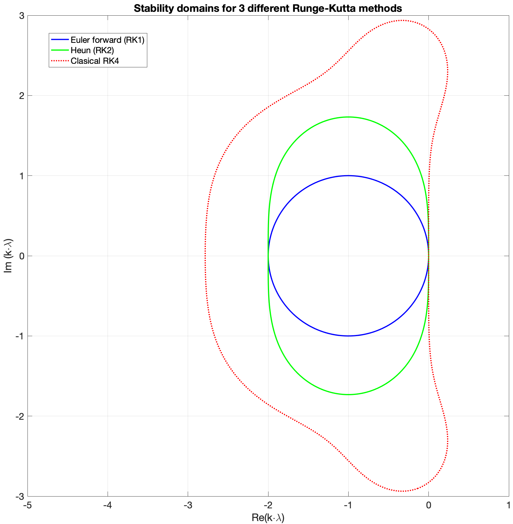
Stability regions of Runge–Kutta methods
The figure below shows the stability regions for three different Runge–Kutta methods. Here \(k\) denotes the time step and \(\lambda\) the coefficient in the test equation:
\[
y' = \lambda y
\]
Exercise 1
Consider the advection-diffusion IBVP,
\[\begin{split}
\begin{array}{lll}
u_t=au_{x} +bu_{xx}, & 0 < x < L, & t> 0,\\
au+2bu_x=0, &x=0,& t > 0,\\
au+2bu_x=0, &x=L,& t > 0,\\
u=f,& 0\le x \le L, & t= 0,\\
\end{array}
\end{split}\]
where \(a\) and \(b>0\) are real constants. You may assume that \(u\) is real too.
a) Prove that the finite difference operator \(D_+D_-\) (obtained by stacking \(D_+\) and \(D_-\)) is a second-order approximation of \(\partial^2/\partial x^2\). The operator is given by
\[
(D_+D_-\mathbf{v})_j = \frac{v_{j-1} - 2v_j + v_{j+1}}{h^2}.
\]
b) Use the energy method to show that the IBVP is well posed.
c) Derive a stable semi-discrete SBP-SAT approximation of the IBVP.
d) Consider using RK4 for time-integration. Approximately how does the largest stable time step depend on the grid spacing \(h\)?
Hint: How do the largest eigenvalues of \(D_1\) and \(D_2\) depend on \(h\)?
Solutions to exercise 1
a) Consider applying the operator to a smooth function \(f=f(x)\). We obtain
\[
(D_+D_- f)_j = \frac{f(x_j-h) - 2f(x_j) + f(x_j+h))}{h^2} .
\]
Taylor-expanding about the point \(x_j\) yields
\[\begin{split}
\begin{aligned}
f(x_j+h) &= f(x_j) + hf'(x_j) + \frac{h^2}{2!}f''(x_j) \\
&+\frac{h^3}{3!}f'''(x_j) + \frac{h^4}{4!}f''''(x_j) + \mathcal{O}(h^5)
\end{aligned}
\end{split}\]
and
\[\begin{split}
\begin{aligned}
f(x_j-h) &= f(x_j) - hf'(x_j) + \frac{h^2}{2!}f''(x_j) \\
&-\frac{h^3}{3!}f'''(x_j) + \frac{h^4}{4!}f''''(x_j) + \mathcal{O}(h^5).
\end{aligned}.
\end{split}\]
Adding everything yields
\[\begin{split}
\begin{aligned}
(D_+D_- f)_j &= \frac{1}{h^2}\left( 2\frac{h^2}{2!}f''(x_j) + 2\frac{h^4}{4!}f''''(x_j) + \mathcal{O}(h^5) \right) \\
&= f''(x_j) + \mathcal{O}(h^2),
\end{aligned}
\end{split}\]
which shows that the finite difference operator is second-order accurate.
b) Multiplying the PDE by \(u\) and integrating in space leads to
\[
\begin{aligned}
(u,u_t)= a(u,u_x) + b(u,u_{xx}).
\end{aligned}
\]
Since \(u\) is assumed to be real, we have
\[
a(u,u_x) = a(u_x,u) = \frac{1}{2} au^2 \big|^L_0
\]
\[
b(u,u_{xx}) = buu_{x}\big|^L_{0} -b(u_x,u_x).
\]
This leads to the energy rate
\[
\frac{1}{2} \frac{\mathrm{d}}{\mathrm{d} t} \lVert u \rVert^2 = \left[ \frac{1}{2} au^2 + buu_{x} \right]^L_0 - b \lVert u_x \rVert^2 \leq \left[ \frac{1}{2} au^2 + buu_{x} \right]^L_0
\]
Using the boundary conditions yields
\[
\frac{1}{2} \frac{\mathrm{d}}{\mathrm{d} t} \lVert u \rVert^2 \leq \left[ \frac{1}{2} au^2 + buu_{x} \right]^L_0 = \left[ \frac{u}{2}( au + 2bu_{x}) \right]^L_0 = 0.
\]
We know that two BC will be needed, since the PDE is second order in space. This set of two BCs yields no growth of \(\lVert u \rVert\) and the IBVP is therefore well posed.
c) A semi-discrete SBP approximation of the IBVP is
\[\begin{split}
\begin{array}{ll}
\mathbf{v}_t=aD_1\mathbf{v} +bD_2\mathbf{v} , & t > 0,\\
(a\mathbf{e}_\ell^T+2b\mathbf{d}_\ell^T)\mathbf{v}=0 , &t > 0,\\
(a\mathbf{e}_r^T+2b\mathbf{d}_r^T)\mathbf{v}=0, & t> 0,\\
\mathbf{v}=f,& t= 0,\\
\end{array}
\end{split}\]
An SBP-SAT approximation of the PDE plus BC is
\[\begin{split}
\begin{aligned}
\mathbf{v}_t &= aD_1\mathbf{v} +bD_2\mathbf{v} \\
&+ \tau_\ell H^{-1} \mathbf{e}_\ell (a\mathbf{e}_\ell^T+2b\mathbf{d}_\ell^T)\mathbf{v} \quad ({\color{red}*}) \\
&+ \tau_r H^{-1} \mathbf{e}_r (a\mathbf{e}_r^T+2b\mathbf{d}_r^T)\mathbf{v},
\end{aligned}
\end{split}\]
where \(\tau_{\ell,r}\) are unknown, scalar penalty parameters. We need to select values of \(\tau_{\ell,r}\) that lead to a stable discretization.
The first step in the discrete energy method is to multiply \(({\color{red}*})\) by \(\mathbf{v}^T H\) from the left, which yields
\[\begin{split}
\begin{aligned}
(\mathbf{v}, \mathbf{v}_t)_H &= a(\mathbf{v}, D_1\mathbf{v})_H + b(\mathbf{v},D_2\mathbf{v})_H \\
&+ \tau_\ell (\mathbf{e}_\ell^T \mathbf{v}) (a\mathbf{e}_\ell^T+2b\mathbf{d}_\ell^T)\mathbf{v} \\
&+ \tau_r (\mathbf{e}_r^T \mathbf{v}) (a\mathbf{e}_r^T+2b\mathbf{d}_r^T)\mathbf{v}.
\end{aligned}
\end{split}\]
Due to the SBP properties of \(D_1\), we have
\[
a(\mathbf{v}, D_1 \mathbf{v})_H = a(\mathbf{e}_r^T \mathbf{v}) (\mathbf{e}_r^T \mathbf{v}) - a(\mathbf{e}_\ell^T \mathbf{v}) (\mathbf{e}_\ell^T \mathbf{v}) - a(D_1 \mathbf{v}, \mathbf{v})_H
\]
Since the inner product is symmetric, we have \((D_1 \mathbf{v}, \mathbf{v})_H = (\mathbf{v}, D_1\mathbf{v})_H\), and therefore
\[
a(\mathbf{v}, D_1 \mathbf{v})_H = \frac{1}{2}a(\mathbf{e}_r^T \mathbf{v}) (\mathbf{e}_r^T \mathbf{v}) - \frac{1}{2} a(\mathbf{e}_\ell^T \mathbf{v}) (\mathbf{e}_\ell^T \mathbf{v}).
\]
The SBP properties of \(D_2\) yield
\[
b(\mathbf{v}, D_2 \mathbf{v})_H = b(\mathbf{e}_r^T \mathbf{v}) (\mathbf{d}_r^T \mathbf{v}) - b(\mathbf{e}_\ell^T \mathbf{v}) (\mathbf{d}_\ell^T \mathbf{v}) - b\mathbf{v}^T M \mathbf{v}.
\]
We obtain the discrete energy rate
\[\begin{split}
\begin{aligned}
\frac{1}{2} \frac{\mathrm{d}}{\mathrm{d} t} \lVert \mathbf{v} \rVert^2_H &= \frac{1}{2}a(\mathbf{e}_r^T \mathbf{v}) (\mathbf{e}_r^T \mathbf{v}) - \frac{1}{2} a(\mathbf{e}_\ell^T \mathbf{v}) (\mathbf{e}_\ell^T \mathbf{v}) \\
&+ b(\mathbf{e}_r^T \mathbf{v}) (\mathbf{d}_r^T \mathbf{v}) - b(\mathbf{e}_\ell^T \mathbf{v}) (\mathbf{d}_\ell^T \mathbf{v}) - b\mathbf{v}^T M \mathbf{v} \\
& + \tau_\ell (\mathbf{e}_\ell^T \mathbf{v}) (a\mathbf{e}_\ell^T+2b\mathbf{d}_\ell^T)\mathbf{v} + \tau_r (\mathbf{e}_r^T \mathbf{v}) (a\mathbf{e}_r^T+2b\mathbf{d}_r^T)\mathbf{v}.
\end{aligned}
\end{split}\]
After some algebra, we see that the choice
\[
\tau_\ell = \frac{1}{2}, \quad \tau_r = -\frac{1}{2},
\]
cancels all the boundary terms. This leads to the discrete energy rate
\[
\frac{1}{2} \frac{\mathrm{d}}{\mathrm{d} t} \lVert \mathbf{v} \rVert^2_H = - b\mathbf{v}^T M \mathbf{v} \leq 0,
\]
which shows that the SBP-SAT approximation is stable. The semi-discrete problem can be written
\[\begin{split}
\begin{array}{ll}
\mathbf{v}_t=aD\mathbf{v} , & t > 0,\\
\mathbf{v}=f,& t= 0,\\
\end{array}
\end{split}\]
where
\[\begin{split}
\begin{aligned}
D = aD_1+bD_2 &+ \frac{1}{2} H^{-1} \mathbf{e}_\ell (a\mathbf{e}_\ell^T+2b\mathbf{d}_\ell^T) \\
&-\frac{1}{2} H^{-1} \mathbf{e}_r (a\mathbf{e}_r^T+2b\mathbf{d}_r^T)
\end{aligned}
\end{split}\]
d) The largest eigenvalue of \(D_1\) is proportional to \(h^{-1}\) whereas the largest eigenvalue of \(D_2\) is proportional to \(h^{-2}\). Hence, for small enough \(h\), the second derivative will dominate and we expect the eigenvalues of the combined operator \(D\) to be proportional to \(h^{-2}\). That is, \(\lambda_{max} = Ch^{-2}\), for some constant C. For stability, we need a time step \(k\) such that
\[
k \lambda_{max} \leq R_{RK4} \Leftrightarrow k Ch^{-2} \leq R_{RK4} \Leftrightarrow k \leq A h^2
\]
where \(R_{RK4} \approx 3\) denotes the “radius” of the RK4 stability region in the direction of the largest eigenvalue, and \(A = R_{RK4}/C\) is a constant. In practice, we may determine an approximate value of \(A\) by computing the eigenvalues of \(D\) for a large mesh size \(h\), in which case computing the eigenvalues is not too expensive.
Exercise 2
Consider the following problem,
\[\begin{split}
\begin{array}{rll}
{\bf u}_{t}= A{\bf u}_x & 0 < x < L , & t > 0,\\
u^{(1)}=0 , &x=0,& t > 0,\\
u^{(1)}+u^{(2)}=0, &x=L,& t > 0,\\
{\bf u}={\bf f},& 0 \le x \le L, & t= 0,\\
\end{array}
\end{split}\]
where \({\bf f}={\bf f}(x)\) is the initial data and
\[\begin{split}
{\bf u}=\begin{bmatrix}
u^{(1)}\\
u^{(2)}\\
\end{bmatrix}, \quad
A=\begin{bmatrix}
2&1 \\
1&0\\
\end{bmatrix}\;.
\end{split}\]
a) Use the energy method to show that the IBVP is well posed. You may assume that the solution is real.
b) Explain why Euler forward (RK1) is not a suitable time-integrator for this IBVP.
Hint: Ignore the boundary conditions and study the periodic problem. What are the eigenvalues of the matrix that discretizes the right-hand side? You might also want to study the ODEs that the Fourier coefficients satisfy.
c) Derive a stable SBP-SAT approximation of the IBVP.
Hint:
For a system of equations it is useful to extend all operators to 2 components. We will use the bar notation for extended operators. We define
\[\begin{split}
\begin{aligned}
\bar{D}_1 &= I_2 \otimes D_1, \quad \bar{H} = I_2 \otimes H, \\
\bar{\mathbf{e}}_\ell &= I_2 \otimes \mathbf{e}_{\ell}, \quad \bar{\mathbf{e}}_r = I_2 \otimes \mathbf{e}_{r},
\end{aligned}
\end{split}\]
where \(I_n\) denotes the \(n\times n\) identity matrix. We also extend the coefficient matrix \(A\) to an \((m+1)\)-point grid:
\[
\bar{A} = A \otimes I_{m+1}.
\]
The SBP property translates to the following property for the extended operators:
\[\begin{split}
\begin{aligned}
(\mathbf{u}, \bar{A} \bar{D}_1 \mathbf{v})_\bar{H} &= (\bar{\mathbf{e}}_r^T \mathbf{u})^* A (\bar{\mathbf{e}}_r^T \mathbf{v}) - (\bar{\mathbf{e}}_\ell^T \mathbf{u})^* A (\bar{\mathbf{e}}_\ell^T \mathbf{v}) \\
&- (\bar{D}_1 \mathbf{u}, \bar{A} \mathbf{v})_{\bar{H}}
\end{aligned}
\end{split}\]
Solutions to exercise 2
a) We use the energy method. Multiplying by \({\bf u}^T\) and integrating in space leads to
\[
({\bf u},{\bf u}_t) = ({\bf u},{\bf A}{\bf u}_x)=[IBP]={\bf u}^T{\bf A}{\bf u}\big|^L_{0}-({\bf u}_x,{\bf A}{\bf u}).
\]
Taking the transpose of the above relation yields
\[
({\bf u}_t,{\bf u}) = ({\bf A}{\bf u}_x,{\bf u})=[{\bf A}={\bf A}^T]=({\bf u}_x,{\bf A}{\bf u}).
\]
Adding the two equations above gives us the energy rate
\[\begin{split}
\frac{\mathrm{d}}{\mathrm{d}t}\|{\bf u}\|^2&={\bf u}^T{\bf A}{\bf u}\big|^L_{0}=2u^{(1)}u^{(1)}+2u^{(1)}u^{(2)}\big|^L_{0}\\
&=2u^{(1)}(u^{(1)}+u^{(2)})\big|^L_{0}=0,
\end{split}\]
where we used the boundary conditions in the last step. There is no way to bound the growth rate with fewer than two boundary conditions, so this is a well-posed set of BC.
b) The Fourier coefficients of the solution to the periodic problem satisfy the ODE (obtained by replacing \(\partial_x\) by \(ik\))
\[
\frac{\mathrm{d} \hat{\mathbf{u}}_k }{\mathrm{d}t} = ik A \hat{\mathbf{u}}_k .
\]
The matrix \(A\) is symmetric and therefore has only real eigenvalues, which implies that the operator \(ikA\) has purely imaginary eigenvalues. This indicates a wave-dominated PDE (which is expected, since the PDE is hyperbolic). Any decent semi-discretization will yield eigenvalues that are similar to those of the continuous problem, i.e. purely imaginary.
We need a time-integrator whose stability region covers the imaginary axis. RK1 is a terrible choice.
c) The SBP approximation of the IBVP is given by
\[\begin{split}
\begin{array}{ll}
\mathbf{v}_t= \bar{A} \bar{D}_1\mathbf{v} , & t > 0,\\
\mathbf{e}_{\ell}^T \mathbf{v}^{(1)} = 0, & t>0, \\
\mathbf{e}_{r}^T(\mathbf{v}^{(1)} + \mathbf{v}^{(2)}) = 0, & t>0, \\
\mathbf{v} = \mathbf{f}, & t=0.
\end{array}
\end{split}\]
An SBP-SAT approximation of the PDE + BC is
\[
\begin{aligned}
\mathbf{v}_t = \bar{A} \bar{D}_1 \mathbf{v} + SAT_{\ell} + SAT_r,
\end{aligned}
\]
where
\[\begin{split}
SAT_\ell = \bar{H}^{-1} \begin{bmatrix}
\tau^{(1)} \mathbf{e}_\ell \\ \tau^{(2)}\mathbf{e}_{\ell}
\end{bmatrix} \mathbf{e}_{\ell}^T \mathbf{v}^{(1)},
\end{split}\]
\[\begin{split}
SAT_r = \bar{H}^{-1} \begin{bmatrix}
\sigma^{(1)} \mathbf{e}_r \\ \sigma^{(2)}\mathbf{e}_r
\end{bmatrix} \mathbf{e}_{r}^T(\mathbf{v}^{(1)} + \mathbf{v}^{(2)}),
\end{split}\]
and \(\tau^{(1,2)}\) and \(\sigma^{(1,2)}\) are scalar parameters that we need to determine such that the semi-discretization is stable.
The discrete energy method starts by multiplying by \(\mathbf{v}^T \bar{H}\) from the left, which yields
\[
(\mathbf{v}, \mathbf{v}_t)_{\bar{H}} = (\mathbf{v}, \bar{A} \bar{D}_1 \mathbf{v})_\bar{H} + \mathbf{v}^T \bar{H} SAT_{\ell} + \mathbf{v}^T \bar{H} SAT_{r} \quad ({\color{blue}*})
\]
Let us try to simplify the terms one by one. We have
\[
(\mathbf{v}, \mathbf{v}_t)_{\bar{H}} = \frac{1}{2} \frac{\mathrm{d}}{\mathrm{d}t} \lVert \mathbf{v} \rVert^2_{\bar{H}}.
\]
The SBP property yields
\[\begin{split}
\begin{aligned}
(\mathbf{v}, \bar{A} \bar{D}_1 \mathbf{v})_\bar{H} &= (\bar{\mathbf{e}}_r^T \mathbf{v})^T A (\bar{\mathbf{e}}_r^T \mathbf{v}) - (\bar{\mathbf{e}}_\ell^T \mathbf{v})^T A (\bar{\mathbf{e}}_\ell^T \mathbf{v}) \\
&- (\bar{D}_1 \mathbf{v}, \bar{A} \mathbf{v})_{\bar{H}}.
\end{aligned}
\end{split}\]
Since \(A\) is symmetric, this is equivalent to
\[\begin{split}
2 (\mathbf{v}, \bar{A} \bar{D}_1 \mathbf{v})_\bar{H} &= (\bar{\mathbf{e}}_r^T \mathbf{v})^T A (\bar{\mathbf{e}}_r^T \mathbf{v}) - (\bar{\mathbf{e}}_\ell^T \mathbf{v})^T A (\bar{\mathbf{e}}_\ell^T \mathbf{v}) \\
&= 2(\mathbf{e}_r^T \mathbf{v}^{(1)})^2 + 2(\mathbf{e}_r^T \mathbf{v}^{(1)})(\mathbf{e}_r^T \mathbf{v}^{(2)}) \\
&- 2(\mathbf{e}_\ell^T \mathbf{v}^{(1)})^2 - 2(\mathbf{e}_\ell^T \mathbf{v}^{(1)})(\mathbf{e}_\ell^T \mathbf{v}^{(2)})
\end{split}\]
To further simplify the notation, we define
\[
v^{(1)}_\ell = \mathbf{e}_\ell^T \mathbf{v}^{(1)}, \quad v^{(2)}_\ell = \mathbf{e}_\ell^T \mathbf{v}^{(2)}, \quad \mathbf{e}_r^T \mathbf{v}^{(1)}, \quad v^{(2)}_r = \mathbf{e}_r^T \mathbf{v}^{(2)},
\]
so that we can write
\[
(\mathbf{v}, \bar{A} \bar{D}_1 \mathbf{v})_\bar{H} = (v_r^{(1)})^2 + v_r^{(1)} v_r^{(2)} - (v_{\ell}^{(1)})^2 - v_{\ell}^{(1)} v_{\ell}^{(2)}.
\]
For the SATs, we obtain
\[\begin{split}
\begin{aligned}
\mathbf{v}^T \bar{H} SAT_{\ell} &= \mathbf{v}^T \begin{bmatrix}
\tau^{(1)} \mathbf{e}_\ell \\
\tau^{(2)}\mathbf{e}_{\ell}
\end{bmatrix} \mathbf{e}_{\ell}^T \mathbf{v}^{(1)} \\
&= \tau^{(1)} (v_{\ell}^{(1)})^2 + \tau^{(2)}v_\ell^{(2)}v_\ell^{(1)},
\end{aligned}
\end{split}\]
\[\begin{split}
\begin{aligned}
\mathbf{v}^T \bar{H} SAT_{r} &= \mathbf{v}^T \begin{bmatrix}
\sigma^{(1)} \mathbf{e}_r \\ \sigma^{(2)}\mathbf{e}_{r}
\end{bmatrix} \mathbf{e}_{r}^T (\mathbf{v}^{(1)}+\mathbf{v}^{(2)})\\
&= \sigma^{(1)} v_r^{(1)} (v_r^{(1)}+v_r^{(2)}) + \sigma^{(2)} v_r^{(2)} (v_r^{(1)}+v_r^{(2)}) .
\end{aligned}
\end{split}\]
We can now write \(({\color{blue}*})\) as
\[
\begin{aligned}
\frac{1}{2} \frac{\mathrm{d}}{\mathrm{d}t} \lVert \mathbf{v} \rVert^2_{\bar{H}} = BT_{\ell} + BT_r,
\end{aligned}
\]
where
\[\begin{split}
\begin{aligned}
BT_\ell &= - (v_{\ell}^{(1)})^2 - v_{\ell}^{(1)} v_{\ell}^{(2)} + \tau^{(1)} (v_{\ell}^{(1)})^2 + \tau^{(2)}v_\ell^{(2)}v_\ell^{(1)} \\
&= (\tau^{(1)}-1) (v_{\ell}^{(1)})^2 + (\tau^{(2)}-1)v_{\ell}^{(1)} v_{\ell}^{(2)}
\end{aligned}.
\end{split}\]
\[\begin{split}
BT_r &= (v_r^{(1)})^2 + v_r^{(1)} v_r^{(2)} + \sigma^{(1)} v_r^{(1)} (v_r^{(1)}+v_r^{(2)}) + \sigma^{(2)} v_r^{(2)} (v_r^{(1)}+v_r^{(2)}) \\
&= (1+\sigma^{(1)})(v_r^{(1)})^2 + (1 + \sigma^{(1)} + \sigma^{(2)}) v_r^{(1)} v_r^{(2)} + \sigma^{(2)}(v_r^{(2)})^2 .
\end{split}\]
We see that \(BT_\ell \leq 0\) if
\[
\tau^{(1)} \leq 1, \quad \tau^{(2)} = 1.
\]
Note that \(\tau^{(1)}\) is a free parameter. It is not obvious what choice is optimal in terms of accuracy, but \(\lvert \tau^{(1)} \rvert >> 1\) would introduce unnecessary stiffness and would probably be a bad choice. We here select \(\tau^{(1)} = 0\).
The expression for \(BT_r\) looks complicated, so let us see if there is a solution for \(\sigma^{(2)}=0\). In this case, we obtain
\[
\begin{aligned}
BT_r &= (1+\sigma^{(1)})(v_r^{(1)})^2 + (1 + \sigma^{(1)}) v_r^{(1)} v_r^{(2)}
\end{aligned}
\]
We obtain \(BT_r=0\) if
\[
\sigma^{(1)} = -1, \quad \sigma^{(1)} = 0.
\]
With these choices,
\[\begin{split}
\begin{aligned}
SAT_\ell &= \bar{H}^{-1} \begin{bmatrix}
0 \cdot \mathbf{e}_\ell \\ \mathbf{e}_{\ell}
\end{bmatrix} \mathbf{e}_{\ell}^T \mathbf{v}^{(1)} \\
&= \bar{H}^{-1} \left( \begin{bmatrix}
0 \\ 1
\end{bmatrix} \otimes \mathbf{e}_\ell \right) ([1, 0] \otimes \mathbf{e}_{\ell}^T) \mathbf{v},
\end{aligned}
\end{split}\]
\[\begin{split}
\begin{aligned}
SAT_r &= \bar{H}^{-1} \begin{bmatrix}
-\mathbf{e}_r \\ 0 \cdot \mathbf{e}_r
\end{bmatrix} \mathbf{e}_{r}^T(\mathbf{v}^{(1)} + \mathbf{v}^{(2)}) \\
&=\bar{H}^{-1} \left( \begin{bmatrix}
-1 \\ 0
\end{bmatrix} \otimes \mathbf{e}_r \right) \left([1, 1] \otimes \mathbf{e}_{r}^T \right) \mathbf{v}
\end{aligned}
\end{split}\]
To summarize, a stable semi-discrete approximation of the IBVP is
\[\begin{split}
\begin{array}{ll}
\mathbf{v}_t= D \mathbf{v} , & t > 0,\\
\mathbf{v} = \mathbf{f}, & t=0,
\end{array}
\end{split}\]
where
\[\begin{split}
\begin{aligned}
D = \bar{A} \bar{D}_1 &+ \bar{H}^{-1} \left( \begin{bmatrix}
0 \\ 1
\end{bmatrix} \otimes \mathbf{e}_\ell \right) ([1, 0] \otimes \mathbf{e}_{\ell}^T) \\
&+ \bar{H}^{-1} \left( \begin{bmatrix}
-1 \\ 0
\end{bmatrix} \otimes \mathbf{e}_r \right) \left([1, 1] \otimes \mathbf{e}_{r}^T \right) ,
\end{aligned}
\end{split}\]