Problem set 2: Finite difference methods
Contents
Problem set 2: Finite difference methods#
Topics covered: Finite difference methods, boundary condition enforcement, stability.
Note: If you miss the problem solving class, you have to submit solutions to 1a)-d) and 2a)-b) in Studium before the deadline.
Preliminaries#
Consider a uniform grid of \(m+1\) points, with grid spacing \(h = \frac{L}{m}\). Let \(\mathbf{e}_{\ell}\) and \(\mathbf{e}_r\) denote the following vectors in \(\mathbb{R}^{m+1}\):
Definition of \(D_1\)#
A difference operator \(D_1\) is a first-derivative SBP operator with quadrature matrix \(H\) if \(H=H^T>0\) and
Definition of \(D_2\)#
A difference operator \(D_2\) approximating \(\partial^2/\partial\,x^2\) is a second-derivative SBP operator if
where \(H=H^T>0\), \(M=M^T \ge 0\), and \(\mathbf{d}_\ell^T v\simeq u_x|_{x=0}\), \(\mathbf{d}_r^T v \simeq u_x |_{x=L}\) are finite difference approximations of the first derivatives at the left and right boundary points.
Discrete inner product#
Let \((\cdot, \cdot)_H\) denote the discrete inner product, defined by
Note that \((\cdot, \cdot)_H\) approximates the \(L^2\) inner product \((\cdot, \cdot)\), since \(H\) is a quadrature operator. In the discrete inner product, the SBP operators satisfy
and
Note the similiarties with the corresponding integration-by-parts formulas.
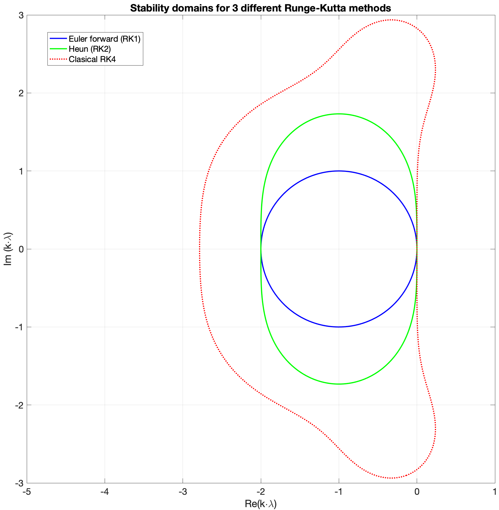
Stability regions of Runge–Kutta methods#
The figure below shows the stability regions for three different Runge–Kutta methods. Here \(k\) denotes the time step and \(\lambda\) the coefficient in the test equation:
Exercise 1#
Consider the advection-diffusion IBVP,
where \(a\) and \(b>0\) are real constants. You may assume that \(u\) is real too.
a) Prove that the finite difference operator \(D_+D_-\) (obtained by stacking \(D_+\) and \(D_-\)) is a second-order approximation of \(\partial^2/\partial x^2\). The operator is given by
b) Use the energy method to show that the IBVP is well posed.
c) Derive a stable semi-discrete SBP-SAT approximation of the IBVP.
d) Consider using RK4 for time-integration. Approximately how does the largest stable time step depend on the grid spacing \(h\)? Hint: How do the largest eigenvalues of \(D_1\) and \(D_2\) depend on \(h\)?
Exercise 2#
Consider the following problem,
where \({\bf f}={\bf f}(x)\) is the initial data and
a) Use the energy method to show that the IBVP is well posed. You may assume that the solution is real.
b) Explain why Euler forward (RK1) is not a suitable time-integrator for this IBVP. Hint: Ignore the boundary conditions and study the periodic problem. What are the eigenvalues of the matrix that discretizes the right-hand side? You might also want to study the ODEs that the Fourier coefficients satisfy.
c) Derive a stable SBP-SAT approximation of the IBVP.
Hint: For a system of equations it is useful to extend all operators to 2 components. We will use the bar notation for extended operators. We define
where \(I_n\) denotes the \(n\times n\) identity matrix. We also extend the coefficient matrix \(A\) to an \((m+1)\)-point grid:
The SBP property translates to the following property for the extended operators: