Applications
MERIT has potential applications in a wide range of mathematical optimization problems. We note that the case-dependent sub-optimality guarantees can be viewed as trust certificates provided along with the approximate solutions, and hence, are of practical importance in decision making scenarios.
To provide an example of MERIT's derivation, in the following, we consider unimodular quadratic programming (UQP), also known as complex quadratic programming. Interestingly, using MERIT one may obtain better performance guarantees for UQP compared to the analytical worst-case guarantees (such as  associated with SDR).
Unimodular Quadratic Programming (UQP)
The NP-hard problem of optimizing a quadratic form over the unimodular vector set arises in a variety of active sensing and communication applications, such as receiver signal-to-noise ratio (SNR) optimization, synthesizing cross ambiguity functions, steering vector estimation, and maximum likelihood (ML) detection. Namely, we study the problem
where  is a given Hermitian matrix, and
  represents the unit circle, i.e.
 .
.
MERIT for UQP
To help the formulation of MERIT, Theorem 1 presents a bijection among the set of matrices leading to the same solution.
Theorem 1.
Let  represent the set of matrices
  for which a given
  is the global optimizer of UQP. Then
 is a convex cone.
For any two vectors
 , the one-to-one mapping

(where  ) holds among the matrices in
  and
and  .
.
It is interesting to note that in light of the above result, the characterization of the cone for any given  leads to a complete characterization of all , , and thus solving any UQP.
While a complete tractable characterization of cannot be expected (due to the NP-hardness of UQP), approximate characterizations of are possible. In the following, our goal is to provide an approximate characterization of the cone which can be used to tackle the UQP problem.
leads to a complete characterization of all , , and thus solving any UQP.
While a complete tractable characterization of cannot be expected (due to the NP-hardness of UQP), approximate characterizations of are possible. In the following, our goal is to provide an approximate characterization of the cone which can be used to tackle the UQP problem.
Theorem 2.
For any given  , let
, let  represent the convex cone of matrices
  where
where  is any real-valued symmetric matrix with non-negative off-diagonal entries. Also let
  represent the convex cone of matrices with
  being their dominant eigenvector (i.e the eigenvector corresponding to the maximal eigenvalue). Then for any
  , there exists
  such that for all
  ,
,
where  stands for the Minkowski sum of the two sets.
An intuitive illustration of the result in Theorem 2 is shown in Fig. 1. Indeed, it can be shown that Theorem 2 is valid even when is a local optimum of the UQP associated with .
 |
Fig. 1. An illustration of the result in Theorem 2. |
 denotes the convex cone of matrices with
 Finally, one can use  as an approximate characterization of noting that the accuracy of such a characterization can be measured by the minimal value of
  . Hereafter, we study a computational method to obtain an which is as small as possible. We also formulate the sub-optimality guarantee for a solution of UQP based on the above approximation.
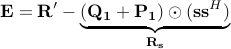
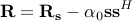
Using the previous results, we build a sequence of matrices (for which the UQP global optima are known) whose distance from the given matrix is decreasing. The proposed iterative approach can be used to solve for the global optimum of UQP or at least to obtain a local optimum (with an upper bound on the sub-optimality of the solution). We know from Theorem 2 that if is a stable point of the UQP associated with then there exist matrices  ,
,  and a scalar such that
 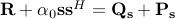 . The latter equation can be rewritten as

where  , and
, and  .
.
We first consider the case of  which corresponds to the global optimality of . Consider the optimization problem:

Note that, as  is a convex cone, the global optimizers
  and
and  for any given can be easily found. On the other hand, the problem of finding an optimal for fixed
  is non-convex and hence more difficult to solve globally.
Note that there exist examples for which the above objective function does not converge to zero. As a result, the proposed method cannot obtain a global optimum of UQP in such cases. However, it is still possible to obtain a local optimum of UQP for some  . To do so, we solve the optimization problem,

with  , for increasing .
Sub-Optimality Analysis
We show how MERIT can provide real-time sub-optimality guarantees and bounds during its iterations. Let (as a result  ) and define
where and .
By construction, the global optimum of the UQP associated with  is . We have that
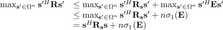
Furthermore,
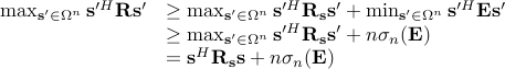
As a result, an upper bound and a lower bound on the objective function for the global optimum of UQP can be obtained at each iteration. Next, suppose that we have to increase in order to obtain the convergence of  to zero. In such a case, we have that
and as a result,

or equivalently,

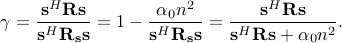
The provided case-dependent sub-optimality guarantee is thus given by
Numerical Examples and Discussion
We use the power method-like iterations, and MERIT, as well as the curvilinear search of with Barzilai-Borwein (BB) step size, to solve an UQP (with  ) based on the same initialization. The resultant UQP objectives along with required times (in sec) versus iteration number are plotted in Fig. 2.
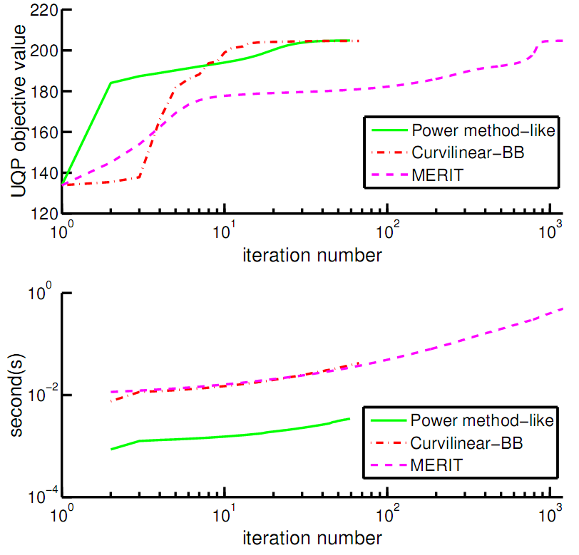 |
Fig. 2. A comparison of power method-like iterations, the curvilinear search with Barzilai-Borwein (BB) step size, and MERIT: (top) the UQP objective; (bottom) the required time for solving an UQP ( |
It can be observed that the power method-like iterations approximate the UQP solution much faster than the employed curvilinear search. On the other hand, both methods are much faster than MERIT. This type of behavior, which is not unexpected, is due to the fact that MERIT is not designed solely for local optimization; indeed, MERIT relies on a considerable over-parametrization in its formulation which is the cost paid for easily derivable sub-optimality guarantees. In general, one may employ the power method-like iterations to obtain a fast approximation of the UQP solution (e.g. by using several initializations), whereas for obtaining sub-optimality guarantees one can resort to MERIT.
Next, we approximate the UQP solutions for  full-rank random positive definite matrices of sizes
  . Inspired by some previous works, we also consider rank-deficient matrices with rank
 . The performance of MERIT for different values of
  is shown in Table 1.
Note that, in general, the provided sub-optimality guarantees
is shown in Table 1.
Note that, in general, the provided sub-optimality guarantees  are considerably larger than
  of SDR. We also employ SDR to solve the same UQPs. In this example, we continue the randomization procedure of SDR until reaching the same UQP objective as for MERIT. A comparison of the computation times of SDR and MERIT can also be found in Table 1.

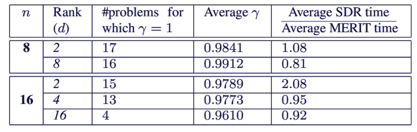 |
Table 1. Comparison of the performance of MERIT and SDR when solving the UQP for |
 and ranks
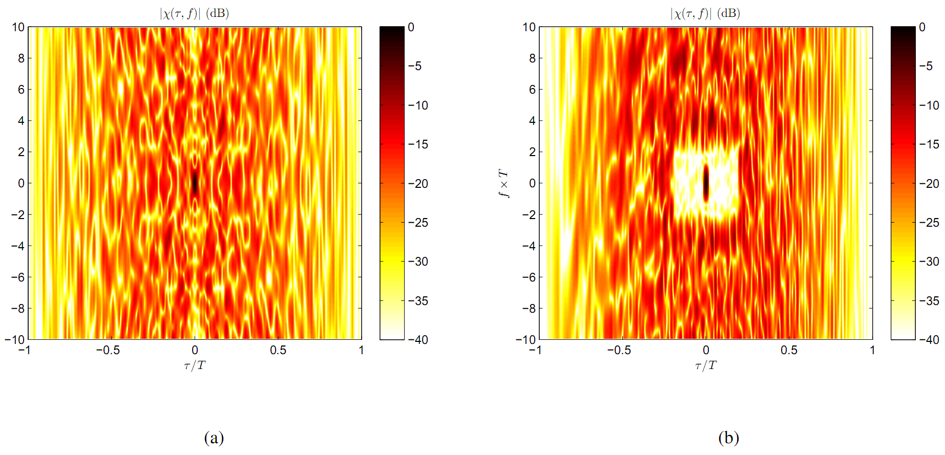 |
Fig. 3. Application of MERIT for designing cross ambiguity functions (CAFs). The normalized CAF modulus for (a) the Bj"orck code of length  (i.e. the initial CAF), and (b) the CAF obtained by MERIT. See the Related Publications for more details.